Java – Refactoring Lightly

There is an interesting comment in the JDK 8 Javadocs that occurs 14 times describing the Arrays.sort() quicksort implementation for primitives, it states:

The sorting algorithm is a Dual-Pivot Quicksort by Vladimir Yaroslavskiy, Jon Bentley, and Joshua Bloch. This algorithm offers O(n log(n)) performance on many data sets that cause other quicksorts to degrade to quadratic performance, and is typically faster than traditional (one-pivot) Quicksort implementations.

Is that statement accurate? A tremendous amount of research has been done on quicksort and dual-pivot quicksort however some of the results are conflicting. Ten years after Java switched to dual-pivot quicksort for primitives other languages have kept an optimized single-pivot implementation instead so the debate is still open as to why Java switched and other languages did not. To better understand the answer and differences I ported the Go single-pivot quicksort to Java and used the Java JDK 8 dual-pivot quicksort code as-is except changing the insertion sort threshold to match Go’s choice at <= 12 elements and using a trivial non-optimized insertion sort algorithm for each.

Conveniently, Go publishes their code, tests & benchmarks so I ported just one test – “func countOps” from sort_test.go and the results were very interesting:

Java 8 Dual-Pivot   q-sort swaps: insertion sort swaps: total swaps
       100 elements:        144 :        154          :        298    
       300 elements:        554 :        474          :       1028    
      1000 elements:       2458 :       1317          :       3775    
      3000 elements:       8964 :       3952          :      12916    
     10000 elements:      36407 :      13317          :      49724    
     30000 elements:     125633 :      39349          :     164982    
    100000 elements:     493535 :     132425          :     625960    
    300000 elements:    1461032 :     400095          :    1861127    
   1000000 elements:    5729345 :    1330589          :    7059934    
Elapsed time:287ms, sort function calls: 325874

Go Single-Pivot
       100 elements:        108 :        245          :        353    
       300 elements:        493 :        488          :        981    
      1000 elements:       2070 :       1576          :       3646    
      3000 elements:       7217 :       4932          :      12149    
     10000 elements:      28355 :      16353          :      44708    
     30000 elements:      96513 :      49123          :     145636    
    100000 elements:     365602 :     163487          :     529089    
    300000 elements:    1209370 :     492204          :    1701574    
   1000000 elements:    4459733 :    1639037          :    6098770    
Elapsed time:256ms, sort function calls: 176646

The input data is the same in both cases from the same random number generator seeded at 0. Most notable is difference in sort function calls, Go uses 149,228 fewer total calls to sort the data! It also completed faster and the code was not even optimized at all for Java so the comparison should favor Java! Also Go wins again comparing number of swaps! Reviewing the optimizations both implementations choose is very interesting. Don’t underestimate how much work has gone into these sorting functions over the years! Go’s implementation is trying to minimize stack depth, partially to avoid switching to heapsort and one optimization they use is to fall through to insertion sort after calling quicksort in a while loop. Here are some lecture notes about this idea.

Go’s slightly simplified sorting code:

func quickSort(data Interface, a, b, maxDepth int) {
    for b-a > 12 { // Use Insertion sort for slices <= 12 elements
        if maxDepth == 0 {
            heapSort(data, a, b)
            return
        }
        maxDepth--
        mlo, mhi := doPivot(data, a, b)
        if mlo-a < b-mhi {
            quickSort(data, a, mlo, maxDepth)
            a = mhi // i.e., quickSort(data, mhi, b)
        } else {
            quickSort(data, mhi, b, maxDepth)
            b = mlo // i.e., quickSort(data, a, mlo)
        }
    }
    if b-a > 1 {
        insertionSort(data, a, b)
    }
}

The dual-pivot quicksort in Java is significantly more complicated and why did they switch to it? A big reason is perhaps that the JDK 6 sort in Java did not take advantage of the optimization of calling insertion sort after quicksort. Interestingly both the JDK6 and Go versions have a similar comment that they are “following Bentley and McIlroy…”

Conclusions

There are some interesting optimizations in both implementations and the newly proposed Java implementation

If the Java & Go approaches adopted some of the ideas currently used in other languages both would potentially improve – there is still fun & interesting work to do. Can you write a tail-recursive style dual-pivot quicksort?
The newer language, Go, publishes the source code, unit tests & benchmarks so open source contributions are much easier. Years ago Java’s approach to the JVM helped create a huge Java ecosystem of shared open source libraries but now the language is showing it’s age in many regards and other languages are likely to improve faster benefitting from better integrating unit tests & benchmarks among other things.
Both implementations take a very different approach to protecting against O(n squared) worst case performance – I may analyze this if people are interested.

The original definition of AVL trees is elegant – all siblings have a maximum height difference of one. Yet surprisingly they have a reputation as complex to implement, particularly the delete operation. Years of research even went into trying to describe simpler balanced binary search trees such as left leaning red-black trees; however, I’ll demonstrate here that AVL trees can be fairly simple to implement with the right approach.

The 2015 paper Rank Balanced Trees describes a new way of thinking about and implementing AVL trees. The simple fact that variations on an idea originally published in 1962 with hand draw binary trees, the original implementation for balanced binary search trees is still relevant today is fascinating. This new rank balanced definition lends itself to at least one simple and one rather complex implementation. We’ll review both in this post. The new approaches to AVL trees stem from the definitions of rank and rank difference.

Rank in an AVL tree is equivalent to height. We’ll define a leaf node as having a rank of zero (it’s non existent null children rank minus one)

Rank difference of node x = Parent Rank(x) – Rank(x)

Therefore, by definition every node except the root in an AVL tree has rank difference of 1 or 2. For the root node, rank difference is undefined.

There are many approaches to the implementation of AVL trees. The recursive approach is popular in textbooks because of simplicity although that approach will sometimes negatively impact performance so we’ll look at bottom-up retracing after inserts via parent references here. The rank and rank difference definitions of AVL trees implemented in this way is, based on my experience, fairly simple (rank) and fairly complicated (store only rank difference at each node).

Rank Balanced AVL Tree Insert

Buckle up! After an insert rank difference (delta rank) during bottom-up retracing can take on one of three values – one, two or three. That’s it. So the bottom-up retracing code:

stops if retracing reaches the root of the tree
stops if rank difference of the node was two before the insert and is now 1 (parent rank therefore stays unchanged)
increments rank if rank difference is equal, then the loop continues
must perform rotations if rank difference of the sibling node was two and would be three if the parent’s rank was incremented. After one or two rotations retracing stops.

Let’s look at the loop, keep in mind we have incremented the rank at node x and are looking up at our parent node to determine which of the above cases to apply.

    private void fixAfterInsertion(Entry<K, V> x) {
	for (Entry<K, V> parent = x.parent;
		parent != null && x.rank + 1 != parent.rank; x.rank++) {
	    if (parent.left == x) { // new node was added on the left
		if (needToRotateRight(parent)) {
		    if (x.left == null || x.rank >= x.left.rank + 2) {
			x.rank--;
			x.right.rank++;
			rotateLeft(x);
		    }
		    parent.rank--;
		    rotateRight(parent);
		    break;
		}
	    } else {
		if (needToRotateLeft(parent)) {
		    if (x.right == null || x.rank >= x.right.rank + 2) {
			x.rank--;
			x.left.rank++;
			rotateRight(x);
		    }
		    parent.rank--;
		    rotateLeft(parent);
		    break;
		}
	    }
	    x = parent;
	    parent = x.parent;
	}
    }

Hmmmm…30 lines of code, actually the logic allows many variations so an easier approach may exist. Anyway let’s review – exit the loop if parent == null or node rank + 1 == parent.rank. Within the loop check on what side the new node was added then check if the rank of our sibling node was two and would be three if the parent rank was incremented meaning rotations are necessary. The methods needToRotateLeft() and needToRotateRight() could be written inline in one line of code. If the delta rank of our sibling means a rotation is necessary then check whether we need to perform a single or double rotation. Adjusting rank for a single rotation means one increment and one decrement of existing ranks as two nodes swap their height in the binary tree. Review the various unit tests for insertion that check single left & right rotations, left-right & right-left rotations and cases which do nothing.

One Extra Bit Per Node Insert Re-tracing

In the above example in Java each node carries the additional overhead of one byte for rank. What if we want to allow only one extra bit per node and never calculate rank difference, just flip the bit when necessary? Then each node would store it’s delta rank of one or two (a boolean in the below code) and the root would have no value defined for delta rank. If a very simple implementation exists so far I haven’t found it so give it a try or implement bit parity as described in the original paper and tell me how it goes. So far for the implementation in my GitHub project the insert with delta rank of one or two looks like this:

    private void fixAfterInsertion(Entry<K, V> x) {
	while (x.deltaR != TWO && x.parent != null) {
	    Entry<K, V> p = x.parent;
	    if (p.left == x) { // node was added on left so check if left side is unbalanced
		Entry<K, V> sibling = p.right;
		if (sibling == null || sibling.deltaR == TWO) { // need to rebalance
		    if (sibling != null)
			sibling.deltaR = ONE;

		    if (x.right != null) {
			 if(x.right.deltaR == ONE) {
			     if (x.left != null) x.left.deltaR = ONE;
			     rotateLeft(x);
			 } else
			     x.right.deltaR = ONE;
		    } 

		    if (p.deltaR == TWO) {  // maintain delta 2 at parent
			p.deltaR = ONE;
			p.left.deltaR = TWO;
		    }
		    rotateRight(p);
		    return;
		} else if (sibling.deltaR == ONE) {
		    sibling.deltaR = TWO;
		}
	    } else { // checking right side heavy
		Entry<K, V> sibling = p.left;
		if (sibling == null || sibling.deltaR == TWO) { // need to rebalance
		    if (sibling != null)
			sibling.deltaR = ONE;

		    if (x.left != null) {
			if (x.left.deltaR == ONE) {
			    if (x.right != null) x.right.deltaR = ONE;
			    rotateRight(x);
			} else
			    x.left.deltaR = ONE;
		    }

		    if (p.deltaR == TWO) {  // maintain delta 2 at parent
			p.deltaR = ONE;
			p.right.deltaR = TWO;
		    }
		    rotateLeft(p);
		    return;
		} else if (sibling.deltaR == ONE) {
		    sibling.deltaR = TWO;
		}
	    }

	    x = x.parent;
	}
	if (x.deltaR == TWO)
	    x.deltaR=ONE;
    }

I’m not going to draw all the tree states which must be understood and tested to correctly preserve rank difference with each rotation but good unit tests are necessary to get the logic right.

AVL Tree Deletes

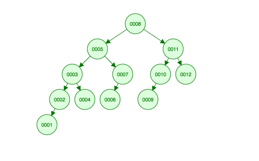
We should expect more than 30 lines of code because there are two more cases to handle. Knuth’s Art of Computer Programming Vol. III discusses AVL trees in detail. With inserts, after a single or double rotation the retracing loop is complete, unfortunately deletes in AVL trees can require O(log n) rotations – rebalancing at more than one level. Why? Consider this Fibonacci tree with twelve elements:

What happens when the node with value 12 is removed? In terms of rank difference the null that replaces node 12 has rank -1, the parent has rank(height) 2 so the temporary rank difference of 3 at node 11 is a violation of AVL tree rules and a right rotation between nodes 10 & 11 is performed. That rotation shortens the height of the tree by one creating a new height violation at the root. So directly reusing the inner loop insert logic may not be possible because after a single or double rotation on insert retracing is done but with deletes rotations may be necessary all the way up to the root of the tree. There is one condition when rotations leave the height of the subtree unchanged:

Balanced Sibling

After Rotation Height Unchanged

In the above example with one additional element compared to the Fibonacci tree, when 120 is removed AVL tree constraints are violated temporarily but the sibling node is balanced so in the case of a right side delete causing an imbalance in the left subtree with a balanced left subtree, retracing can stop after one right rotation.

Overall there are three conditions which stop retracing:

The loop reaches the root
A single rotation where the sibling node was balanced
A delete from a balanced tree – height at the parent remains unchanged so stop.

So one way to implement this logic is:

private void fixAfterDeletion(Entry<K, V> parent, Entry<K, V> sibling, Entry<K, V> node) {
	if (sibling == null)  // remove sibling null check inside loop by testing once here
	    sibling = EMPTY_NODE;
	int balance = sibling.rank - node.rank;

	while (balance != 1) { // balance == 1 means prior to delete parent was balanced, break;
	    if (balance == 0) {// side of delete was taller, decrement and continue
		parent.rank--;
	    } else if (parent.left == sibling) {
		parent.rank -= 2;
		int siblingBalance = rank(sibling.right) - rank(sibling.left);
		if (siblingBalance == 0) { // parent height unchanged after rotate so break
		    sibling.rank++;
		    parent.rank++;
		    rotateRight(parent);
		    break;
		} else if (siblingBalance > 0) {
		    sibling.right.rank++;
		    sibling.rank--;
		    rotateLeft(sibling);
		}
		rotateRight(parent);
		parent = parent.parent;
	    } else { // delete on left
		parent.rank -= 2;
		int siblingBalance = rank(sibling.right) - rank(sibling.left);
		if (siblingBalance == 0) { // parent height unchanged after rotate so break
		    sibling.rank++;
		    parent.rank++;
		    rotateLeft(parent);
		    break;
		} else if (siblingBalance < 0) {
		    sibling.left.rank++;
		    sibling.rank--;
		    rotateRight(sibling);
		}
		rotateLeft(parent);
		parent = parent.parent;
	    }

	    if (parent.parent == null)
		return;
	    node = parent;
	    parent = parent.parent;
	    sibling = (parent.left == node) ? parent.right : parent.left;
	    balance = sibling.rank - node.rank;
	}

Manageable. What about AVL deletes with one extra bit per node that stores rank difference? Send me a link to the code if you write it, I haven’t yet.

Conclusion

Alternatives such as red-black trees have worse theoretical height bounds to AVL trees and often more complicated insert/delete operations; therefore, Looking for alternatives to AVL trees because AVL trees are too complex to implement or have presumed slower insert/delete operations is a rather futile endeavor.

dmcmanam@gmail.com.